SCI图片复现：热图+折线图+堆积柱状图

代码包含三个主要部分：绘制热图、绘制折线图和绘制堆积柱状图，并最后将它们合并并保存为PDF文件。在细节上，我会进行一些修改以增强可读性和图形的美观度。

首先，我们需要加载必要的库。如果尚未安装这些库，需要首先在R中安装它们。

# 加载所需的库
library(ggplot2)
library(tidyverse)
library(ComplexHeatmap)
library(RColorBrewer)
library(patchwork)

接下来，我们生成热图所需的数据并绘制热图：

# 热图数据构建
sample_ids <- factor(c(paste0("P", 1:17), 
                       paste0("M", 1:10), 
                       paste0("C", 1:3)), 
                     levels = c(paste0("P", 1:17), 
                                paste0("M", 1:10), 
                                paste0("C", 1:3)))

heatmap_data <- data.frame(
  Data_source = sample(c("GSE131907", "GSE123904"), 30, replace = T),
  Sample_Origins = rep(c("Primary", "Distant Metastasis", "Chemotherapy"), c(15,12,3)),
  Smoking = sample(c("Current Smoker", "Former Smoker", "Never Smoker"), 30, replace = T),
  EGFR = sample(c("EGFR Mutation", "WT"), 30, replace = T),
  Stages = sample(paste0("Stage", 1:4), 30, replace = T)
)

rownames(heatmap_data) <- sample_ids

# 定义颜色
color_scheme <- list(
  Data_source = c("#ff8969", "#e9cd50"),
  Sample_Origins = c("#0e9cc4", "#f3734e", "#c05a9c"),
  Smoking = c("#bed4ad", "#bdd3ac", "#96c18c"), 
  EGFR = c("#f7d4b5","#fcf5dd"),
  Stages = c("#feeff4", "#f5cedc", "#f7afcc", "#ec75a7")
)

color_vector <- unlist(color_scheme)

names(color_vector) <- c("GSE131907", "GSE123904",
                         "Primary", "Distant Metastasis", "Chemotherapy",
                         "Current Smoker", "Former Smoker", "Never Smoker",
                         "EGFR Mutation", "WT",
                         paste0("Stage", 1:4))

# 绘制热图
heatmap_plot <- Heatmap(t(heatmap_data),
                        col = color_vector,
                        row_names_side = "left",
                        row_names_gp = gpar(fontsize = 10),
                        rect_gp = gpar(col = "white", lwd = 1),
                        show_column_names = F,
                        show_heatmap_legend = F)

# 保存热图为图片
png("heatmap.png", width = 1000, height = 160)
draw(heatmap_plot)
dev.off()

# 读取热图图片
heatmap_img <- readPNG("heatmap.png")
heatmap_grob <- rasterGrob(heatmap_img)

然后，我们生成折线图所需的数据并绘制折线图：

# 折线图数据构建
line_data <- data.frame(
  x = sample_ids,
  value = c(sort(sample(1:10, 18, replace = T)),
            sort(sample(4:12, 9, replace = T)),
            sort(sample(6:10, 3, replace = T))
  ))

# 绘制折线图
line_plot <- ggplot(line_data, aes(x, value)) +
  geom_point(size = 2) +
  geom_line(size = 1, group = 1) +
  scale_y_continuous(breaks = seq(0, 12, 2)) +
  ylab("log2(Malignant Cell Number)") +
  theme_classic() +
  theme(panel.grid = element_blank(),
        axis.line.x = element_blank(),
        axis.text.x = element_blank(),
        axis.ticks.x = element_blank(),
        axis.title.x = element_blank(),
        axis.line.y = element_line(size = 1),
        axis.ticks.y = element_line(size = 1))

接下来，我们生成堆积柱状图所需的数据并绘制堆积柱状图：

# 堆积柱状图数据构建
bar_data <- data.frame()

for (i in 1:30) {
  cell_category <- sample(3:6, 1)
  bar_data_tmp <- data.frame(
    x = rep(sample_ids[i], cell_category),
    values = sample(20:100, cell_category),
    group = paste0("group", 1:cell_category))
  bar_data_tmp$proportion <- bar_data_tmp$values/sum(bar_data_tmp$values)
  bar_data <- rbind(bar_data, bar_data_tmp)
}

# 绘制堆积柱状图
bar_plot <- ggplot(bar_data)+
  geom_bar(aes(x, proportion*100, fill = group),
           color = "white", width = 1, size = 1,
           stat = "identity", position = "stack")+
  scale_fill_brewer(palette = "Set3")+
  theme_classic()+
  ylab("Cell Proportion(%)")+
  theme(panel.grid = element_blank(),
        legend.position = "none",
        axis.line.x = element_blank(),
        axis.ticks.x = element_blank(),
        axis.title.x = element_blank(),
        axis.line.y = element_line(size = 1),
        axis.ticks.y = element_line(size = 1))

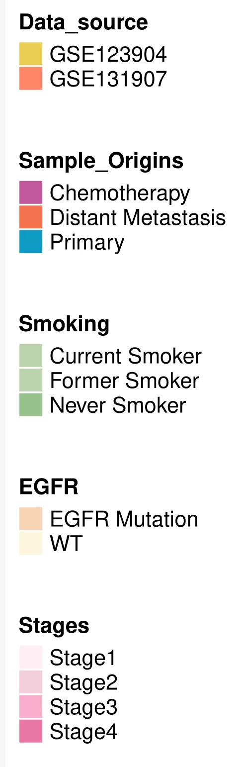
生成图例

# 自定义图例：
legend_list = list()
for(i in 1:ncol(heatmap_data)){
  unique_values = sort(unique(heatmap_data[,i]))
  title = colnames(heatmap_data)[i]
  legend_list[[i]] = Legend(seq(0, 1, length.out = length(unique_values)), labels = unique_values,
                    title = title, legend_gp = gpar(fill = cols_vec[unique_values]))
}

# 把各个图例合并在一起
packed_legend = packLegend(list = legend_list, 
                direction = "vertical", 
                column_gap = unit(5, "mm"), 
                row_gap = unit(1, "cm"))

# 保存图例为PDF
pdf("legend.pdf", height = 6, width = 1.5)
draw(packed_legend)
dev.off()

保存

# 创建图例
legend <- grid::textGrob("Legend", gp = grid::gpar(fontsize = 14, fontface = "bold"))

# 组合图像，并指定每个子图的高度
final_plot <- gridExtra::grid.arrange(legend, heatmap_grob, line_plot, bar_plot, ncol = 1, heights = c(1, 3, 2, 2))

# 保存为 PDF
ggsave("final_plot.pdf", final_plot, width = 10, height = 15)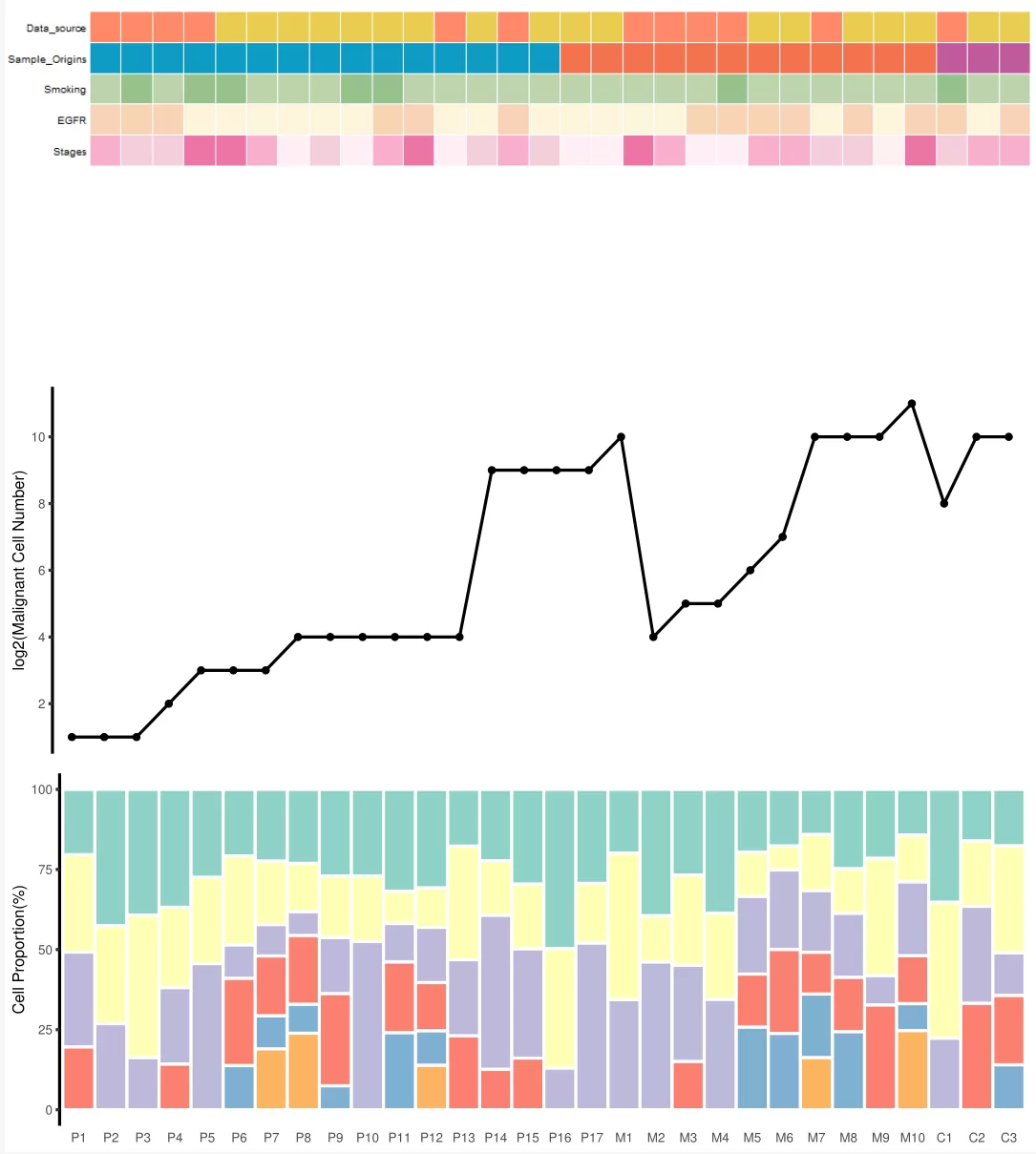

使用AI进行调整美化，